How to find alpha on a lineweaver burk plot – How to find alpha on a Lineweaver-Burk plot? Prepare to embark on a journey through the enzymatic world, where we’ll unravel the secrets hidden within this fascinating graphical representation. This exploration promises to be insightful, equipping you with the knowledge to decipher the enigmatic alpha value and its implications.
The Lineweaver-Burk plot, a cornerstone of enzyme kinetics, transforms the Michaelis-Menten equation into a linear format. This allows for a straightforward determination of key kinetic parameters, including the apparent Michaelis constant (alpha). We will delve into the specifics, guiding you through the process with clarity and precision.
Understanding the Lineweaver-Burk Plot
Yo, fam! This Lineweaver-Burk plot is like the ultimate cheat code for figuring out enzyme kinetics. It’s a way to visualize how enzymes work, and it’s super helpful for finding important info like the Michaelis-Menten constant (Km) and the maximum reaction velocity (Vmax). Get ready to level up your bio knowledge!This plot is a linear transformation of the Michaelis-Menten equation, making it easier to spot trends and calculate those crucial constants.
It’s like taking a complex equation and simplifying it into something you can totally grasp. Let’s dive in!
Derivation from the Michaelis-Menten Equation, How to find alpha on a lineweaver burk plot
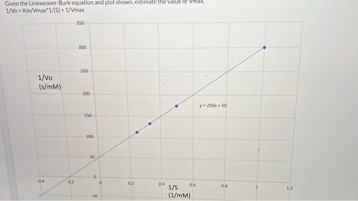
The Michaelis-Menten equation describes how the rate of an enzyme-catalyzed reaction depends on the substrate concentration. It’s a fundamental equation in enzyme kinetics. This equation, 1/v = (Km/Vmax)(1/[S]) + 1/Vmax, is the key to unlocking the Lineweaver-Burk plot. By rearranging the Michaelis-Menten equation, we get a linear equation of the form y = mx + b.
This transformation is what allows us to plot 1/v versus 1/[S].
Relationship between Intercepts and Constants
The Lineweaver-Burk plot’s x-intercept represents the substrate concentration ([S]) where the reaction rate (v) is half of its maximum value (Vmax/2). This is directly related to the Michaelis-Menten constant (Km). Mathematically, the x-intercept is -1/Km. The y-intercept, on the other hand, is directly equal to 1/Vmax. This means you can easily read off the values of Km and Vmax from the plot.
Identifying Slope and Y-Intercept
Let’s say you’ve got a Lineweaver-Burk plot. To find the slope, you’d choose two points on the line, calculate the change in y over the change in x. The y-intercept is where the line crosses the y-axis; it’s the value of y when x is zero. Finding these values gives you the crucial info for understanding the enzyme’s behavior.
Comparison with Other Graphical Representations
Other plots, like the Michaelis-Menten plot itself, and the Eadie-Hofstee plot, also show enzyme kinetics. The Lineweaver-Burk plot is linear, making it easier to determine Km and Vmax. However, it’s crucial to remember that the Lineweaver-Burk plot can sometimes distort the data at higher substrate concentrations. Other plots might be better suited for certain analyses.
Key Features Summary
| Feature | Description | Equation |
|---|---|---|
| Equation | A linear transformation of the Michaelis-Menten equation. | 1/v = (Km/Vmax)(1/[S]) + 1/Vmax |
| X-intercept | Represents -1/Km, crucial for determining the Michaelis-Menten constant. | -1/Km |
| Y-intercept | Represents 1/Vmax, providing the maximum reaction velocity. | 1/Vmax |
| Slope | Represents Km/Vmax, linking the Michaelis-Menten constant to the maximum reaction velocity. | Km/Vmax |
Determining Alpha from the Plot
Yo, fam! So, you’ve cracked the Lineweaver-Burk plot, right? Now, let’s get down to brass tacks and figure out how to extract that alpha value, also known as the apparent Michaelis constant (Km). This alpha value tells us how much the enzyme’s activity changes when something messes with it. It’s crucial for understanding enzyme kinetics and how inhibitors or activators affect enzyme function.The Lineweaver-Burk plot is a graph of 1/v versus 1/[S].
The alpha value is deeply embedded in this graph. It’s not just some random number—it’s a key to unlocking how much the enzyme’s affinity for its substrate changes. We’ll break it down, step by step, so you can totally crush these problems.
Interpreting the Alpha Value
The alpha value is directly related to the x-intercept of the Lineweaver-Burk plot. The x-intercept represents the point where 1/v is zero, which corresponds to the substrate concentration ([S]) at which the reaction rate (v) is maximal. This allows us to calculate the apparent Michaelis constant (Km) which can be different when compared to the Km in the absence of an inhibitor.
This apparent Km is represented by alpha Km. This means the alpha value, in a sense, is a scaling factor that tells us how much the apparent Km changes compared to the Km without the inhibitor. Changes in alpha are super important in understanding how inhibitors or activators affect the enzyme.
Finding the Apparent Km (alpha Km)
To find the alpha value, we need to pinpoint specific points on the Lineweaver-Burk plot. The alpha value can be determined from the x-intercept of the plot. The x-intercept of the Lineweaver-Burk plot is equal to -1/Km. Once you find the x-intercept, you can calculate the apparent Km (alpha Km).
Deriving Alpha from the Intercept or Slope
The alpha value can be derived from the x-intercept or the slope of the Lineweaver-Burk plot. The x-intercept is a crucial point because it directly corresponds to the apparent Km. To calculate the alpha value, you take the x-intercept value for the inhibited reaction and divide it by the x-intercept value for the uninhibited reaction. This gives you a ratio that directly represents the alpha value.
Impact of Inhibitors on Alpha
Inhibitors, like competitive or non-competitive inhibitors, drastically alter the alpha value. For instance, competitive inhibitors increase the apparent Km, resulting in a higher alpha value. Non-competitive inhibitors, on the other hand, affect the maximum velocity, which alters the y-intercept, but the apparent Km stays the same. Knowing how inhibitors impact alpha is key to understanding how they affect enzyme function.
Steps to Find Alpha
| Step | Description | Calculation | Interpretation |
|---|---|---|---|
| 1 | Determine the x-intercept (1/Km) for the uninhibited reaction. | Read the value from the graph. | This gives you the original Michaelis constant (Km) value. |
| 2 | Determine the x-intercept (1/alpha Km) for the inhibited reaction. | Read the value from the graph. | This gives you the apparent Michaelis constant (alpha Km) value for the inhibited reaction. |
| 3 | Calculate alpha. | alpha = (1/alpha Km) / (1/Km) = Km / alpha Km | This ratio tells you how much the apparent Km has changed due to the inhibitor. A higher alpha value indicates a larger apparent Km, suggesting the inhibitor is making the enzyme less effective at binding the substrate. |
Practical Applications and Considerations
Yo, fam, let’s dive into the real-world uses of the Lineweaver-Burk plot and the lowdown on its limitations. This ain’t just some academic exercise; it’s about figuring out how enzymes work in different situations. We’ll break down how to use it to analyze enzyme kinetics, spot potential problems, and compare it to other methods.This plot, while helpful, ain’t perfect.
Understanding its strengths and weaknesses is crucial for accurate interpretations. It’s like using a cool new app – you gotta know how to use it right to get the results you need. We’ll also show you how to make one from scratch, using real data. This ain’t some theoretical stuff, this is how scientists actually study enzymes.
Applying the Lineweaver-Burk Plot in Different Scenarios
The Lineweaver-Burk plot is a powerful tool for studying how different substrates affect enzyme activity. For example, imagine you’re investigating how varying substrate concentrations influence an enzyme’s catalytic efficiency. You’d measure reaction rates at different substrate concentrations and then plot them on the Lineweaver-Burk graph. The slope and y-intercept will reveal crucial information about the enzyme’s behavior, like the Michaelis constant (Km) and maximum velocity (Vmax).
By comparing Lineweaver-Burk plots for different substrates, you can easily visualize how these substrates impact the enzyme’s kinetic parameters. This helps researchers understand enzyme-substrate interactions and optimize reaction conditions.
Limitations of the Lineweaver-Burk Plot
The Lineweaver-Burk plot, while useful, has limitations. One major drawback is its sensitivity to experimental errors, especially at low substrate concentrations. Outliers in your data can heavily skew the plot’s results. Also, the linearization process can exaggerate small errors, making the extracted values less precise than other methods. It’s like trying to zoom in too much on a blurry picture – you’ll see more artifacts than details.
Another key point is that it can be misleading when dealing with enzyme kinetics that aren’t hyperbolic.
Comparing the Lineweaver-Burk Plot with Other Methods
Different methods exist for analyzing enzyme kinetics. The Lineweaver-Burk plot, while popular, has its rivals. The Eadie-Hofstee plot is another linearization method, but it has a similar susceptibility to errors at low substrate concentrations. The Hanes-Woolf plot, on the other hand, minimizes the impact of errors at high substrate concentrations. Each method has its strengths and weaknesses.
The choice of method depends on the specific research question and the characteristics of the enzyme being studied.
Procedure for Generating a Lineweaver-Burk Plot from Raw Data
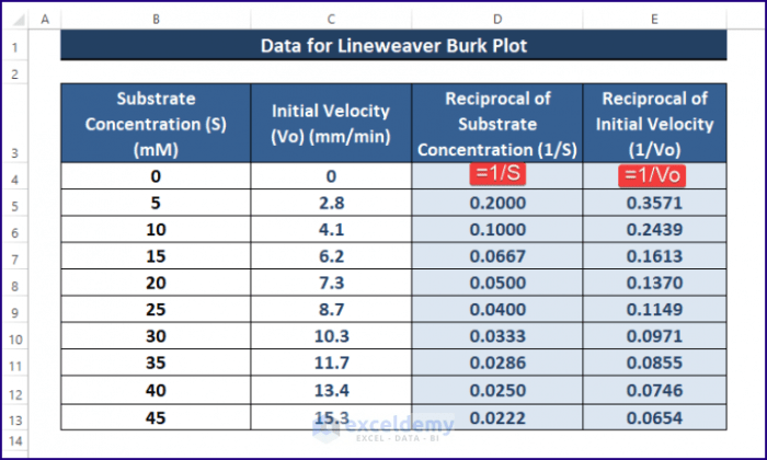
To create a Lineweaver-Burk plot from scratch, you need raw data. This typically involves measuring the reaction rate (velocity) at various substrate concentrations. First, calculate the reciprocal of both the substrate concentration and the reaction rate (velocity). Plot these reciprocals (1/[S]) on the x-axis and (1/V) on the y-axis. You should get a straight line.
The slope and y-intercept of this line will give you the Michaelis-Menten constant and the maximum velocity. This method is commonly used by researchers to determine enzyme kinetics.
Contrasting the Lineweaver-Burk Plot with Other Graphical Representations
| Graphical Representation | Strengths | Weaknesses ||—|—|—|| Lineweaver-Burk Plot | Easy to interpret Km and Vmax | Highly sensitive to errors, especially at low substrate concentrations; distorts the curvature of the Michaelis-Menten plot. || Eadie-Hofstee Plot | Provides a direct estimate of Km and Vmax | Similar sensitivity to errors at low substrate concentrations as the Lineweaver-Burk plot. || Hanes-Woolf Plot | Minimizes the impact of errors at high substrate concentrations | Less straightforward to interpret than Lineweaver-Burk or Eadie-Hofstee plots.
|| Michaelis-Menten Plot | Clearly shows the hyperbolic relationship between substrate concentration and reaction rate. | Determining Km and Vmax from this plot requires more complex calculations. |
Final Conclusion: How To Find Alpha On A Lineweaver Burk Plot
In conclusion, mastering the Lineweaver-Burk plot for determining alpha unlocks a powerful tool for analyzing enzyme kinetics. By understanding the plot’s properties, calculating the apparent Michaelis constant, and interpreting inhibitor effects, you gain valuable insight into enzyme behavior. Remember, though, the plot has its limitations, and comparing it with other methods remains crucial for a complete understanding.
FAQ Explained
What is the significance of alpha in enzyme kinetics?
Alpha represents the apparent Michaelis constant (Km) under specific conditions, often indicating the influence of inhibitors or different substrates on the enzyme’s activity.
Can the Lineweaver-Burk plot be used for all enzyme kinetic studies?
While valuable, the Lineweaver-Burk plot has limitations. Its linearity assumption might not hold true for all enzyme systems, making other methods like the Eadie-Hofstee plot potentially more suitable in certain cases.
How do inhibitors affect the alpha value on the Lineweaver-Burk plot?
Inhibitors shift the plot, altering the slope and y-intercept, which, in turn, modifies the apparent Michaelis constant (alpha). Understanding these shifts is key to interpreting the inhibitor’s impact on enzyme activity.
What are the potential pitfalls of using the Lineweaver-Burk plot?
The Lineweaver-Burk plot’s linearity assumption can be problematic at high substrate concentrations. Also, experimental errors can disproportionately affect the calculated values, so caution and critical analysis are necessary.
